
ggcorrplot function#
In this notebook, we’ll describe the python package ggcorrplot for displaying easily a correlation matrix using ‘plotnine’.
mtcars dataset#
the mtcars data set will be used in the following python code. The function cor_pmat [in ggcorrplot] computes a matrix of correlation p-values
[1]:
#disable warnings
from warnings import simplefilter, filterwarnings
simplefilter(action='ignore', category=FutureWarning)
filterwarnings("ignore")
[2]:
#load mtcars dataset form plotnine
from plotnine.data import mtcars
print(mtcars)
                   name   mpg  cyl   disp   hp  drat     wt   qsec  vs  am  \
0             Mazda RX4  21.0    6  160.0  110  3.90  2.620  16.46   0   1
1         Mazda RX4 Wag  21.0    6  160.0  110  3.90  2.875  17.02   0   1
2            Datsun 710  22.8    4  108.0   93  3.85  2.320  18.61   1   1
3        Hornet 4 Drive  21.4    6  258.0  110  3.08  3.215  19.44   1   0
4     Hornet Sportabout  18.7    8  360.0  175  3.15  3.440  17.02   0   0
5               Valiant  18.1    6  225.0  105  2.76  3.460  20.22   1   0
6            Duster 360  14.3    8  360.0  245  3.21  3.570  15.84   0   0
7             Merc 240D  24.4    4  146.7   62  3.69  3.190  20.00   1   0
8              Merc 230  22.8    4  140.8   95  3.92  3.150  22.90   1   0
9              Merc 280  19.2    6  167.6  123  3.92  3.440  18.30   1   0
10            Merc 280C  17.8    6  167.6  123  3.92  3.440  18.90   1   0
11           Merc 450SE  16.4    8  275.8  180  3.07  4.070  17.40   0   0
12           Merc 450SL  17.3    8  275.8  180  3.07  3.730  17.60   0   0
13          Merc 450SLC  15.2    8  275.8  180  3.07  3.780  18.00   0   0
14   Cadillac Fleetwood  10.4    8  472.0  205  2.93  5.250  17.98   0   0
15  Lincoln Continental  10.4    8  460.0  215  3.00  5.424  17.82   0   0
16    Chrysler Imperial  14.7    8  440.0  230  3.23  5.345  17.42   0   0
17             Fiat 128  32.4    4   78.7   66  4.08  2.200  19.47   1   1
18          Honda Civic  30.4    4   75.7   52  4.93  1.615  18.52   1   1
19       Toyota Corolla  33.9    4   71.1   65  4.22  1.835  19.90   1   1
20        Toyota Corona  21.5    4  120.1   97  3.70  2.465  20.01   1   0
21     Dodge Challenger  15.5    8  318.0  150  2.76  3.520  16.87   0   0
22          AMC Javelin  15.2    8  304.0  150  3.15  3.435  17.30   0   0
23           Camaro Z28  13.3    8  350.0  245  3.73  3.840  15.41   0   0
24     Pontiac Firebird  19.2    8  400.0  175  3.08  3.845  17.05   0   0
25            Fiat X1-9  27.3    4   79.0   66  4.08  1.935  18.90   1   1
26        Porsche 914-2  26.0    4  120.3   91  4.43  2.140  16.70   0   1
27         Lotus Europa  30.4    4   95.1  113  3.77  1.513  16.90   1   1
28       Ford Pantera L  15.8    8  351.0  264  4.22  3.170  14.50   0   1
29         Ferrari Dino  19.7    6  145.0  175  3.62  2.770  15.50   0   1
30        Maserati Bora  15.0    8  301.0  335  3.54  3.570  14.60   0   1
31           Volvo 142E  21.4    4  121.0  109  4.11  2.780  18.60   1   1

    gear  carb
0      4     4
1      4     4
2      4     1
3      3     1
4      3     2
5      3     1
6      3     4
7      4     2
8      4     2
9      4     4
10     4     4
11     3     3
12     3     3
13     3     3
14     3     4
15     3     4
16     3     4
17     4     1
18     4     2
19     4     1
20     3     1
21     3     2
22     3     2
23     3     4
24     3     2
25     4     1
26     5     2
27     5     2
28     5     4
29     5     6
30     5     8
31     4     2
We set name as rownames
[3]:
# Set name as index
mtcars = mtcars.set_index("name")
print(mtcars)
                      mpg  cyl   disp   hp  drat     wt   qsec  vs  am  gear  \
name
Mazda RX4            21.0    6  160.0  110  3.90  2.620  16.46   0   1     4
Mazda RX4 Wag        21.0    6  160.0  110  3.90  2.875  17.02   0   1     4
Datsun 710           22.8    4  108.0   93  3.85  2.320  18.61   1   1     4
Hornet 4 Drive       21.4    6  258.0  110  3.08  3.215  19.44   1   0     3
Hornet Sportabout    18.7    8  360.0  175  3.15  3.440  17.02   0   0     3
Valiant              18.1    6  225.0  105  2.76  3.460  20.22   1   0     3
Duster 360           14.3    8  360.0  245  3.21  3.570  15.84   0   0     3
Merc 240D            24.4    4  146.7   62  3.69  3.190  20.00   1   0     4
Merc 230             22.8    4  140.8   95  3.92  3.150  22.90   1   0     4
Merc 280             19.2    6  167.6  123  3.92  3.440  18.30   1   0     4
Merc 280C            17.8    6  167.6  123  3.92  3.440  18.90   1   0     4
Merc 450SE           16.4    8  275.8  180  3.07  4.070  17.40   0   0     3
Merc 450SL           17.3    8  275.8  180  3.07  3.730  17.60   0   0     3
Merc 450SLC          15.2    8  275.8  180  3.07  3.780  18.00   0   0     3
Cadillac Fleetwood   10.4    8  472.0  205  2.93  5.250  17.98   0   0     3
Lincoln Continental  10.4    8  460.0  215  3.00  5.424  17.82   0   0     3
Chrysler Imperial    14.7    8  440.0  230  3.23  5.345  17.42   0   0     3
Fiat 128             32.4    4   78.7   66  4.08  2.200  19.47   1   1     4
Honda Civic          30.4    4   75.7   52  4.93  1.615  18.52   1   1     4
Toyota Corolla       33.9    4   71.1   65  4.22  1.835  19.90   1   1     4
Toyota Corona        21.5    4  120.1   97  3.70  2.465  20.01   1   0     3
Dodge Challenger     15.5    8  318.0  150  2.76  3.520  16.87   0   0     3
AMC Javelin          15.2    8  304.0  150  3.15  3.435  17.30   0   0     3
Camaro Z28           13.3    8  350.0  245  3.73  3.840  15.41   0   0     3
Pontiac Firebird     19.2    8  400.0  175  3.08  3.845  17.05   0   0     3
Fiat X1-9            27.3    4   79.0   66  4.08  1.935  18.90   1   1     4
Porsche 914-2        26.0    4  120.3   91  4.43  2.140  16.70   0   1     5
Lotus Europa         30.4    4   95.1  113  3.77  1.513  16.90   1   1     5
Ford Pantera L       15.8    8  351.0  264  4.22  3.170  14.50   0   1     5
Ferrari Dino         19.7    6  145.0  175  3.62  2.770  15.50   0   1     5
Maserati Bora        15.0    8  301.0  335  3.54  3.570  14.60   0   1     5
Volvo 142E           21.4    4  121.0  109  4.11  2.780  18.60   1   1     4

                     carb
name
Mazda RX4               4
Mazda RX4 Wag           4
Datsun 710              1
Hornet 4 Drive          1
Hornet Sportabout       2
Valiant                 1
Duster 360              4
Merc 240D               2
Merc 230                2
Merc 280                4
Merc 280C               4
Merc 450SE              3
Merc 450SL              3
Merc 450SLC             3
Cadillac Fleetwood      4
Lincoln Continental     4
Chrysler Imperial       4
Fiat 128                1
Honda Civic             2
Toyota Corolla          1
Toyota Corona           1
Dodge Challenger        2
AMC Javelin             2
Camaro Z28              4
Pontiac Firebird        2
Fiat X1-9               1
Porsche 914-2           2
Lotus Europa            2
Ford Pantera L          4
Ferrari Dino            6
Maserati Bora           8
Volvo 142E              2
Compute a correlation matrix#
[4]:
# Compute a correlation matrix
corr = mtcars.corr()
print(corr.round(4))
         mpg     cyl    disp      hp    drat      wt    qsec      vs      am  \
mpg   1.0000 -0.8522 -0.8476 -0.7762  0.6812 -0.8677  0.4187  0.6640  0.5998
cyl  -0.8522  1.0000  0.9020  0.8324 -0.6999  0.7825 -0.5912 -0.8108 -0.5226
disp -0.8476  0.9020  1.0000  0.7909 -0.7102  0.8880 -0.4337 -0.7104 -0.5912
hp   -0.7762  0.8324  0.7909  1.0000 -0.4488  0.6587 -0.7082 -0.7231 -0.2432
drat  0.6812 -0.6999 -0.7102 -0.4488  1.0000 -0.7124  0.0912  0.4403  0.7127
wt   -0.8677  0.7825  0.8880  0.6587 -0.7124  1.0000 -0.1747 -0.5549 -0.6925
qsec  0.4187 -0.5912 -0.4337 -0.7082  0.0912 -0.1747  1.0000  0.7445 -0.2299
vs    0.6640 -0.8108 -0.7104 -0.7231  0.4403 -0.5549  0.7445  1.0000  0.1683
am    0.5998 -0.5226 -0.5912 -0.2432  0.7127 -0.6925 -0.2299  0.1683  1.0000
gear  0.4803 -0.4927 -0.5556 -0.1257  0.6996 -0.5833 -0.2127  0.2060  0.7941
carb -0.5509  0.5270  0.3950  0.7498 -0.0908  0.4276 -0.6562 -0.5696  0.0575

        gear    carb
mpg   0.4803 -0.5509
cyl  -0.4927  0.5270
disp -0.5556  0.3950
hp   -0.1257  0.7498
drat  0.6996 -0.0908
wt   -0.5833  0.4276
qsec -0.2127 -0.6562
vs    0.2060 -0.5696
am    0.7941  0.0575
gear  1.0000  0.2741
carb  0.2741  1.0000
Correlation matrix p-value#
[5]:
# Compute a matrix of correlation p-values
from ggcorrplot import cor_pmat
p_mat = cor_pmat(mtcars)
print(p_mat.round(4))
         mpg     cyl    disp      hp    drat      wt    qsec      vs      am  \
mpg   0.0000  0.0000  0.0000  0.0000  0.0000  0.0000  0.0171  0.0000  0.0003
cyl   0.0000  0.0000  0.0000  0.0000  0.0000  0.0000  0.0004  0.0000  0.0022
disp  0.0000  0.0000  0.0000  0.0000  0.0000  0.0000  0.0131  0.0000  0.0004
hp    0.0000  0.0000  0.0000  0.0000  0.0100  0.0000  0.0000  0.0000  0.1798
drat  0.0000  0.0000  0.0000  0.0100  0.0000  0.0000  0.6196  0.0117  0.0000
wt    0.0000  0.0000  0.0000  0.0000  0.0000  0.0000  0.3389  0.0010  0.0000
qsec  0.0171  0.0004  0.0131  0.0000  0.6196  0.3389  0.0000  0.0000  0.2057
vs    0.0000  0.0000  0.0000  0.0000  0.0117  0.0010  0.0000  0.0000  0.3570
am    0.0003  0.0022  0.0004  0.1798  0.0000  0.0000  0.2057  0.3570  0.0000
gear  0.0054  0.0042  0.0010  0.4930  0.0000  0.0005  0.2425  0.2579  0.0000
carb  0.0011  0.0019  0.0253  0.0000  0.6212  0.0146  0.0000  0.0007  0.7545

        gear    carb
mpg   0.0054  0.0011
cyl   0.0042  0.0019
disp  0.0010  0.0253
hp    0.4930  0.0000
drat  0.0000  0.6212
wt    0.0005  0.0146
qsec  0.2425  0.0000
vs    0.2579  0.0007
am    0.0000  0.7545
gear  0.0000  0.1290
carb  0.1290  0.0000
Correlation matrix visualization#
[6]:
from ggcorrplot import ggcorrplot
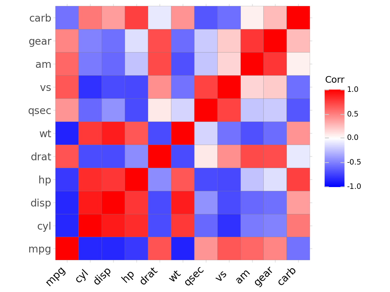
method = “squared” (default)#
[7]:
# method = "square" (default)
p = ggcorrplot(corr)
p
[7]:
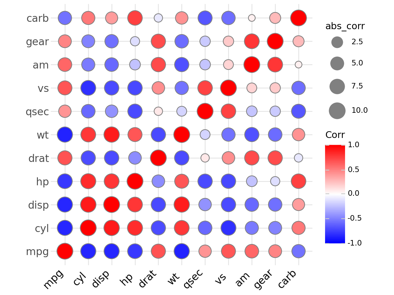
method = “circle”#
[8]:
# method = "circle"
p = ggcorrplot(corr,method = "circle")
p
[8]:
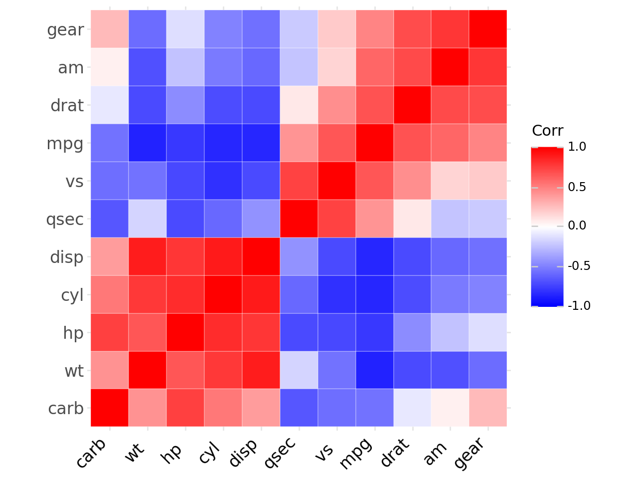
Reordering the correlation matrix#
[9]:
# using hierarchical clustering
p = ggcorrplot(corr,
               hc_order = True,
               outline_color = "white")
p
[9]:
Types of correlogram layout#
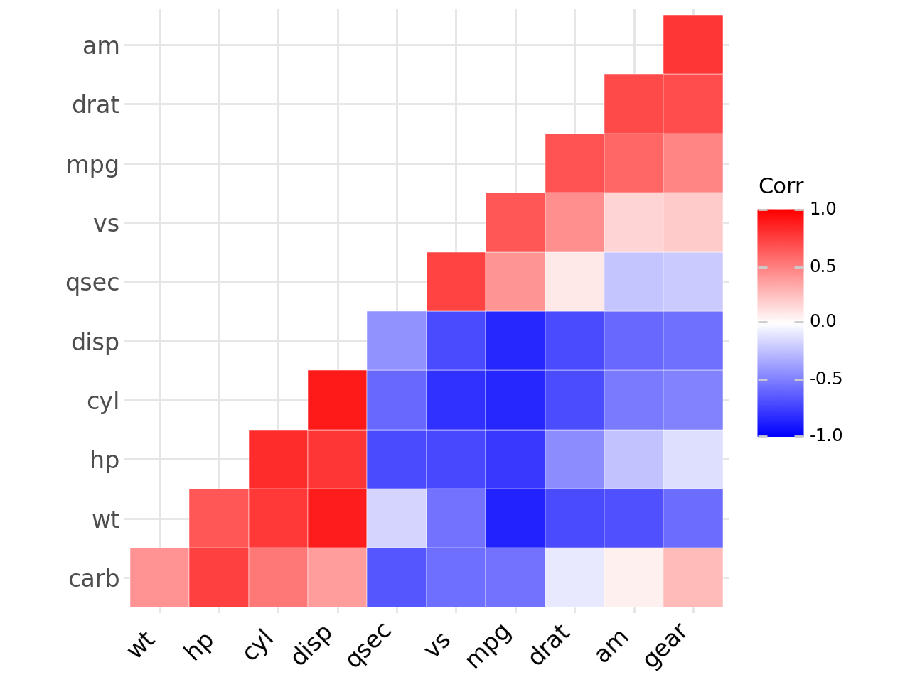
Get the lower triangle#
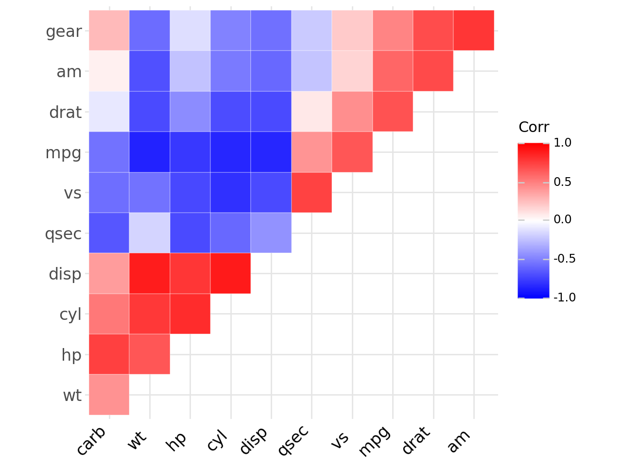
[10]:
# Get the lower triangle
p = ggcorrplot(corr,
               hc_order = True,
               type = "lower",
               outline_color = "white")
p
[10]:
Get the upper triangle#
[11]:
# Get the upper triangle
p = ggcorrplot(corr,
               hc_order = True,
               type = "upper",
               outline_color = "white")
p
[11]:
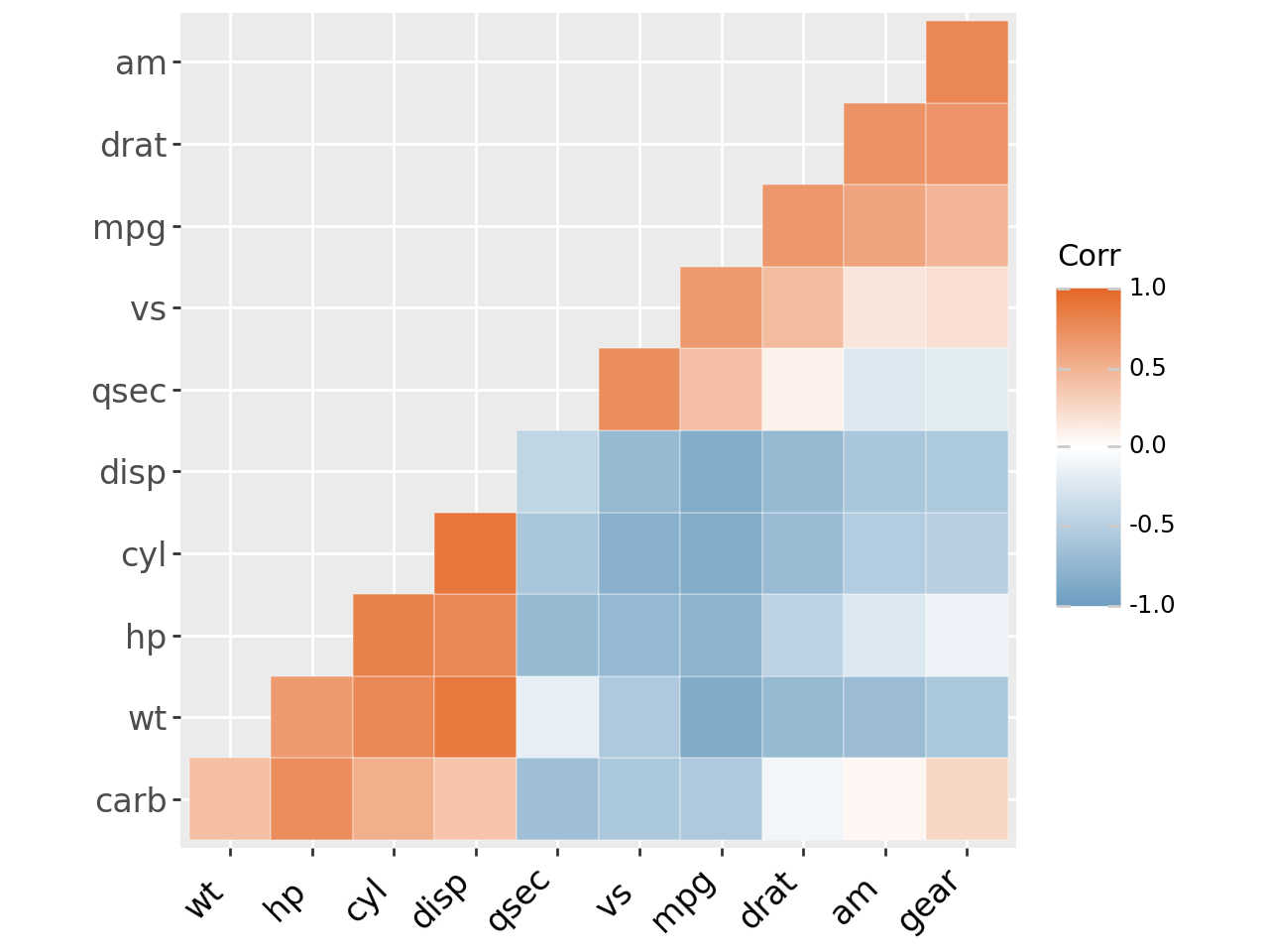
Change colors and theme#
[12]:
# Argument colors
from plotnine import theme_gray
p = ggcorrplot(corr,
               hc_order = True,
               type = "lower",
               outline_color = "white",
               ggtheme = theme_gray(),
               colors = ("#6D9EC1", "white", "#E46726"))
p
[12]:
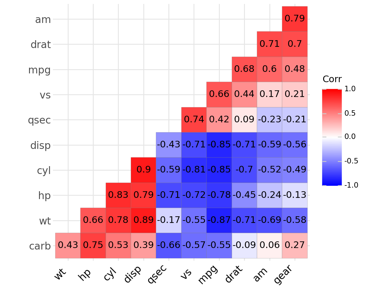
Add correlation coefficients#
[13]:
# argument label = True
p = ggcorrplot(corr,
               hc_order = True,
               type = "lower",
               label = True)
p
[13]:
Add correlation significance level#
[14]:
# Argument p_mat
# Barring the no significant coefficient
p = ggcorrplot(corr,
               hc_order = True,
               type = "lower",
               p_mat = p_mat)
p
[14]:

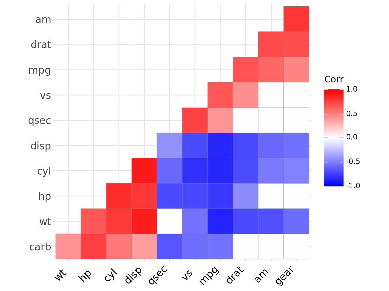
Leave blank on no significant coefficient#
[15]:
# Leave blank on no significant coefficient
p = ggcorrplot(corr,
               p_mat = p_mat,
               hc_order = True,
               type = "lower",
               insig = "blank")
p
[15]:
Using original data#
[16]:
#usinf original dataset
p = ggcorrplot(mtcars,
               matrix_type="completed")
p
[16]:
